Session 1.1.5 – Logistic Regression
The Problem: Predicting Mortality in Healthcare
In healthcare, we often need to predict binary outcomes—events that either happen or don't happen:
- Will this patient survive their hospital stay?
- Will this patient develop a complication?
- Does this patient have a particular disease?
Vizient Mortality Prediction: A Real-World Example
Vizient is a healthcare performance improvement company that provides risk-adjusted mortality models to help hospitals benchmark their outcomes. These models use logistic regression to predict the probability of in-hospital mortality based on patient characteristics.

Consider gastrointestinal (GI) bleeding—a common, serious condition that requires rapid assessment and intervention. Predicting mortality risk helps clinicians:
- Identify high-risk patients who need intensive monitoring
- Guide resource allocation decisions
- Compare outcomes across hospitals after adjusting for patient risk
- Support shared decision-making with patients and families
Learning Objectives
By the end of this session, you will be able to:
-
Explain why linear regression fails for binary outcomes - Understand the fundamental limitations of linear regression when predicting probabilities and binary events, including the problem of predictions outside the [0,1] range
-
Understand the logistic regression model and link function - Describe how logistic regression transforms a linear combination of predictors into probabilities using the logit link function, creating an S-shaped curve that ensures probabilities stay between 0 and 1
-
Interpret logistic regression coefficients as odds ratios - Explain what coefficients in a logistic regression model mean in clinical context, understanding how each predictor affects the odds (and probability) of the outcome, using the Vizient-like GI bleed mortality model as an example
-
Recognize the advantages and limitations of logistic regression - Identify strengths (handles binary outcomes, interpretable odds ratios, well-calibrated probabilities) and limitations (assumes linearity in log-odds, requires adequate sample size, sensitive to class imbalance) when applied to healthcare prediction problems
1. Why Linear Regression Fails for Binary Outcomes
The Problem with Continuous Predictions
Imagine trying to predict whether a patient with GI bleeding will die using linear regression. We might model:
Mortality = β₀ + β₁(Age) + β₂(Sepsis) + ...
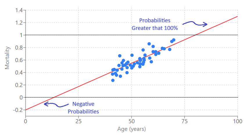
But what does this produce? A continuous number that could be:
- Negative (e.g., -0.3)—what does "negative mortality" mean?
- Greater than 1 (e.g., 1.5)—what does "150% mortality" mean?
These predictions are meaningless for binary outcomes. We need probabilities that are:
- Bounded between 0 and 1
- Interpretable as the chance an event will occur
Visual Comparison
Let's see how linear and logistic regression differ when predicting binary outcomes:
Linear Regression
Logistic Regression
Notice how:
- Linear regression can produce predictions outside [0,1] and doesn't capture the S-shaped relationship
- Logistic regression produces probabilities bounded between 0 and 1, with a natural S-curve that reflects how risk changes with predictor values
2. Logistic Regression: The Model
The Core Idea
Logistic regression solves the binary outcome problem by:
- Modeling the log-odds (logit) of the outcome as a linear function of predictors
- Transforming the log-odds back to probabilities using the logistic function
This ensures probabilities always stay between 0 and 1, while still allowing us to use a linear combination of predictors.
The Logit Link Function
The logit (log-odds) is defined as:
logit(p) = ln(p / (1-p))
Where:
- p = probability of the outcome (e.g., mortality)
- p / (1-p) = the odds of the outcome
- ln(odds) = the log-odds or logit
The logit can range from -∞ to +∞, making it perfect for linear modeling.
The Logistic Regression Formula
The transformation from linear log-odds to S-shaped probabilities is the heart of logistic regression. Let's explore this visually:
Watch how a linear relationship in log-odds space becomes an S-curve in probability space:
Step 1: The Logit Function
logit(p) = -6 + 0.1 × age
We start with a linear equation for the logit (log-odds) of probability p.
This transformation creates the characteristic S-shaped curve that:
- Approaches 0 as logit → -∞
- Approaches 1 as logit → +∞
- Is steepest when p ≈ 0.5 (logit ≈ 0)
3. Vizient-like GI Bleed Mortality Model
Here's an illustrative example of how a Vizient-like model might predict mortality in GI bleeding patients. This is a simplified, educational example (not the actual proprietary Vizient model):
The Model Equation
The model predicts mortality probability using logistic regression with the following equation:
logit(p) = -7.0 + 0.055 × (Age) + 0.20 × (Male) + 0.60 × (Emergency) + 0.90 × (ICU_24h) + 0.08 × (ElixScore) + 0.70 × (CHF_POA) + 0.55 × (CKD_POA) + 1.10 × (Sepsis_POA) + 1.40 × (Vent_24h) + 0.65 × (Creatinine_high) + 0.85 × (Lactate_high)
Then convert to probability:
p = 1 / (1 + exp(-logit(p)))
Explore how patient characteristics affect predicted mortality risk using this interactive calculator. Adjust the patient characteristics on the left to see how the model calculates:
- The logit value (log-odds)
- The predicted mortality probability (as a percentage)
- The contribution of each predictor to the final risk estimate
4. Interpreting Coefficients as Odds Ratios
What Do Coefficients Mean?
In logistic regression, coefficients tell us how predictors affect the log-odds of the outcome. But it's often more intuitive to think in terms of odds ratios.
Converting Coefficients to Odds Ratios
For a coefficient β, the odds ratio is: OR = exp(β)
The odds ratio tells us: "How many times more likely is the outcome when the predictor increases by 1 unit (or is present vs. absent)?"
Interpreting the Vizient-like Model Coefficients
Let's interpret some coefficients from our GI bleed mortality model:
Coefficient: 0.055 for Age
- Odds Ratio per year: exp(0.055) = 1.057
- Meaning: Each additional year of age increases the odds of mortality by 5.7% (or multiplies odds by 1.057)
- Clinical interpretation: Age is a continuous risk factor—older patients have incrementally higher risk, with the effect compounding over decades
Coefficient: 1.10 for Sepsis_POA
- Odds Ratio: exp(1.10) = 3.00
- Meaning: Patients with sepsis present-on-admission have 3.00 times higher odds of mortality
- Clinical interpretation: Sepsis is a life-threatening condition that substantially increases mortality risk in GI bleeding patients
Important Notes on Interpretation
-
Odds vs. Probability: Odds ratios describe relative changes in odds, not probabilities. A 2x increase in odds doesn't mean a 2x increase in probability (the relationship is non-linear)
-
Holding other variables constant: Like in linear regression, each coefficient represents the effect of that predictor while holding all other predictors constant
-
Interaction effects: The model assumes predictors act independently. In reality, some combinations (e.g., sepsis + mechanical ventilation) might have synergistic effects not captured by simple additive terms
5. Evaluation Metrics: AUC, Sensitivity, and Specificity
The ROC curve plots sensitivity (True Positive Rate) vs. 1 - specificity (False Positive Rate) across all classification thresholds. The Area Under the ROC Curve (AUC) summarizes discrimination:
- AUC = 0.5: Random guessing
- AUC = 0.7-0.8: Acceptable
- AUC = 0.8-0.9: Excellent
- AUC > 0.9: Outstanding
At any threshold, predictions form a confusion matrix with four categories: True Positives (TP), False Positives (FP), True Negatives (TN), and False Negatives (FN). Key metrics:
- Sensitivity (Recall): TP / (TP + FN) - How well does the model identify positive cases?
- Specificity: TN / (TN + FP) - How well does the model avoid false alarms?
- Accuracy: (TP + TN) / Total - Overall correctness (can be misleading with imbalanced data)
There's a trade-off between sensitivity and specificity: lower thresholds increase sensitivity but decrease specificity. The optimal threshold depends on clinical context (e.g., screening vs. confirmatory tests).
Interact with this demonstration to see how the ROC curve, confusion matrix, and classification metrics change as you adjust the classification threshold:
6. Advantages and Limitations of Logistic Regression
When Logistic Regression Works Well
✅ Good for:
- Binary outcomes (mortality, complications, diagnoses)
- When interpretability is important (odds ratios are clinically meaningful)
- When you have a moderate number of predictors
- When relationships are approximately linear in log-odds space
- When you need well-calibrated probability estimates
When to Consider Alternatives
❌ Consider other methods when:
- You have very few events (rare outcomes) relative to predictors
- Relationships are highly non-linear in log-odds space
- You have many predictors relative to sample size (consider regularization)
- You need to model complex interactions automatically (consider machine learning)
- You have clustered or longitudinal data (consider mixed-effects models)
Summary
Key Takeaways
-
Linear regression fails for binary outcomes - It can produce predictions outside [0,1] and assumes constant variance, which doesn't hold for binary data. We need a method that constrains predictions to valid probability ranges.
-
Logistic regression uses the logit link function - It models the log-odds (logit) as a linear combination of predictors, then transforms to probabilities using the logistic function. This creates an S-shaped curve that ensures probabilities stay between 0 and 1.
-
Coefficients represent odds ratios - Each coefficient tells us how a predictor affects the odds of the outcome. The odds ratio = exp(coefficient) describes the multiplicative effect on odds. This allows us to quantify risk factors and understand which patient characteristics matter most for outcomes like mortality.
-
Logistic regression has strengths and limitations - It's interpretable, handles binary outcomes well, and produces calibrated probabilities. However, it assumes linearity in log-odds, requires adequate sample size, and may oversimplify complex relationships. Understanding these trade-offs helps you know when logistic regression is appropriate and when to consider alternatives.
Questions for Reflection
-
Why can't we simply constrain linear regression predictions to [0,1] and use that for binary outcomes? What problems would this approach still have?
-
In the Vizient-like model, why might sepsis (coefficient 1.10) have a smaller effect than mechanical ventilation (coefficient 1.40)? What clinical factors could explain this?
-
How would you interpret an odds ratio of 2.0 for a continuous predictor like age? How does this differ from interpreting an odds ratio of 2.0 for a binary predictor like "male"?
-
What additional variables might improve a GI bleed mortality prediction model? What about interaction terms (e.g., sepsis × age)?
-
How might the coefficients in this model differ if you were predicting mortality in a different patient population (e.g., pediatric patients, elective surgery patients)?
References
-
Hosmer, D. W., Lemeshow, S., & Sturdivant, R. X. (2013). Applied logistic regression (3rd ed.). John Wiley & Sons.
-
Steyerberg, E. W. (2019). Clinical prediction models: A practical approach to development, validation, and updating (2nd ed.). Springer.
-
Vizient. (n.d.). Clinical Data Base and Resource Manager. Retrieved from Vizient website.